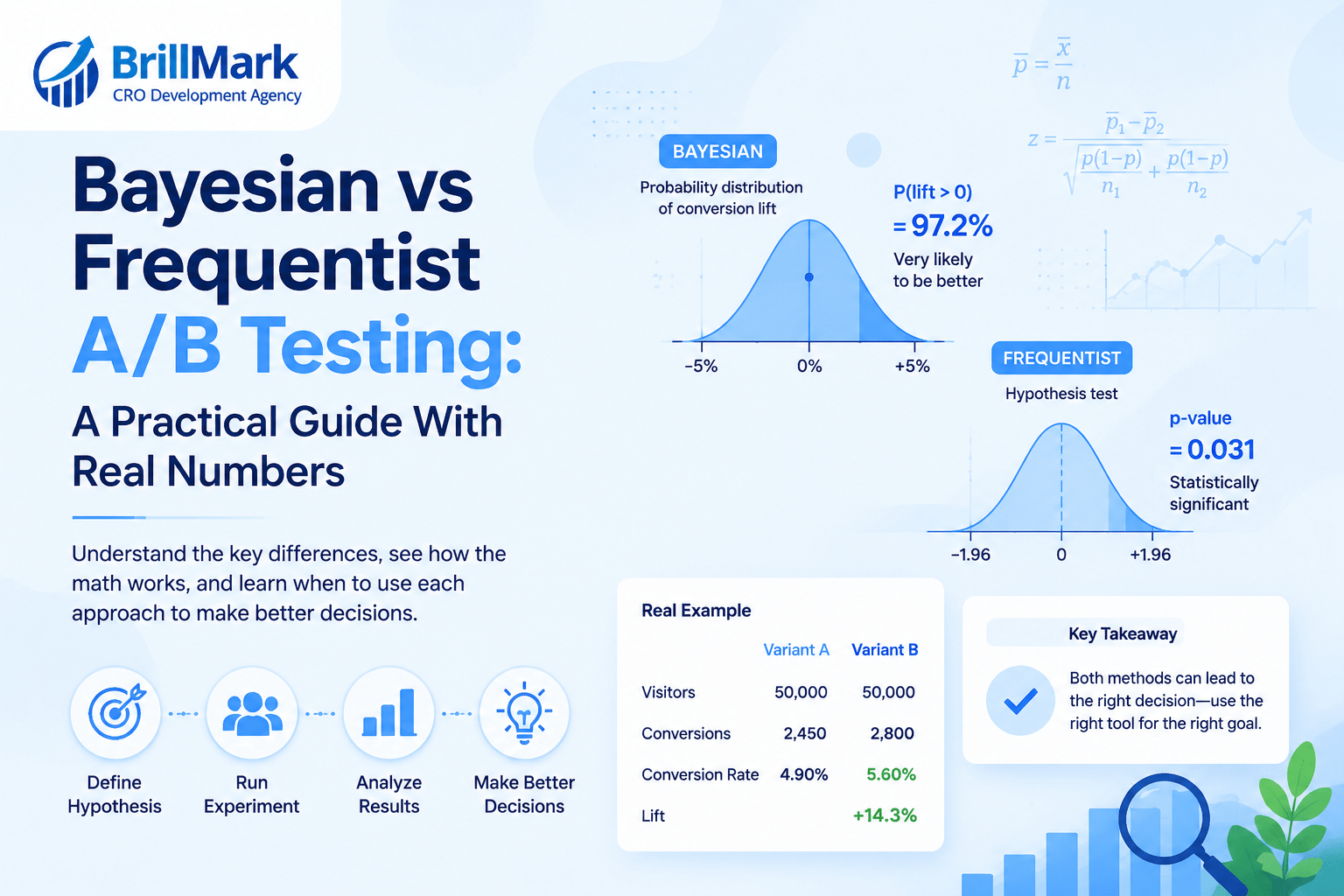
Two analysts look at the same A/B test (Bayesian vs Frequentist). One says “not significant, p = 0.066, keep the control.” The other says “96.7% probability the variant wins, ship it.” Neither is lying. Neither made an arithmetic error. They are reading the same 36,000 visitors through two different definitions of the word probability, and that difference decides which tests you ship, which you kill, and how long you wait.
This guide walks through both frameworks using one worked example with real, reproducible numbers. You will see exactly where the two methods agree (more often than most articles admit), exactly where they diverge, and which one fits your traffic, your stakeholders, and your risk tolerance.
What is inferential statistics, and why does A/B testing need it?
Inferential statistics is the practice of using a limited sample to conclude a larger population you cannot fully observe. In A/B testing, you show two versions to 36,000 visitors over two weeks, but the decision you are making applies to every visitor for the next twelve months. The gap between what you measured and what you are deciding is the entire problem.
Here is the part that gets skipped in most CRO training: you never observe a conversion rate. You observe a count. If 720 out of 18,000 visitors converted, “4.00%” is not the truth about your checkout page; it is one noisy estimate of an underlying rate you will never see directly. Run the identical page next week, and you might get 4.2%. Or 3.8%. That wobble is sampling variation, and it exists even when nothing about your site has changed.
Inferential statistics gives you tools to separate signal from that wobble. Both the frequentist and Bayesian frameworks do this job. They disagree on something more fundamental than method:
| Question | Frequentist answer | Bayesian answer |
| What is probability? | The long-run frequency of an outcome across many repeated trials | A degree of belief, updated as evidence arrives |
| Is the true conversion rate a fixed number? | Yes – fixed but unknown | It is described by a distribution of plausible values |
| What is random? | The data (your sample) | Your belief about the parameter |
Everything downstream p-values, confidence intervals, credible intervals, expected loss follows from that one philosophical split. Understanding it is the difference between running tests and reading dashboards.
What is Frequentist A/B testing?
Frequentist A/B testing evaluates whether observed data would be surprising under the assumption that your variant made no difference. You pre-commit to a sample size, run the test to completion, then calculate a p-value: the probability of seeing a result at least this extreme if the null hypothesis were true. Below your threshold, usually 0.05, you reject the null.
The frequentist workflow
- State a null hypothesis. There is no difference between control and variant.
- Set your error tolerances. Significance level (α, typically 0.05) caps how often you’ll falsely declare a winner. Power (typically 80%) sets how often you’ll detect a real effect of a given size.
- Choose a minimum detectable effect (MDE). The smallest lift worth catching.
- Calculate the required sample size. This is non-negotiable;e it must happen before traffic starts.
- Run to that sample size. Do not look.
- Compute the p-value and confidence interval. Decide.
Step 5 is where nearly every commercial testing programme breaks down, and we’ll quantify the damage later in this guide.
What a p-value actually is
A p-value is the probability of your data given the null hypothesis: P(data | no effect). It is emphatically not the probability that the null hypothesis is true given your data. Those two quantities are different, and the confusion between them is the single most common statistical error in conversion optimization.
A confidence interval carries the same inverted logic. “95% confidence interval: +0.6% to +20.1%” does not mean there is a 95% probability the true lift sits in that range. It means that if you repeated this experiment endlessly, 95% of the intervals you constructed this way would contain the true value. The guarantee is about the procedure, not about your specific result.
Sample size is the real constraint. nt
Frequentist planning forces an uncomfortable conversation before you write any code. Here is what a 4.00% baseline conversion rate actually requires, at 80% power and α = 0.05 two-tailed:
| Minimum detectable effect (relative) | Visitors per variant | Total visitors |
| 5% lift (4.00% → 4.20%) | 154,304 | 308,608 |
| 10% lift (4.00% → 4.40%) | 39,475 | 78,950 |
| 15% lift (4.00% → 4.60%) | 17,943 | 35,885 |
| 20% lift (4.00% → 4.80%) | 10,316 | 20,632 |
Notice the shape of that table. Halving the effect you want to detect roughly quadruples the traffic you need. Most sites that “can’t get significant results” don’t have a statistics problem — they have an arithmetic problem, and this table is it.
What is Bayesian A/B testing?
Bayesian A/B testing treats each variant’s conversion rate as a distribution of plausible values rather than a single unknown constant. You start with a prior belief, update it with observed data using Bayes’ theorem, and end with a posterior distribution. From that posterior you read direct answers: the probability the variant beats control, a credible interval for the lift, and the expected cost of being wrong.
The Bayesian workflow
- Specify a prior for each variant’s conversion rate: what you believed before the test.
- Collect data.
- Update to a posterior using Bayes’ theorem.
- Read the decision metrics from the posterior.
For binary conversion metrics, step 3 is arithmetic rather than heavy computation. The Beta distribution is conjugate to the binomial, which means the update is a one-line operation:
Posterior = Beta(α_prior + conversions, β_prior + non-conversions)
Control: Beta(1 + 720, 1 + 17,280)
Variant: Beta(1 + 790, 1 + 17,210)
That is the whole engine. A uniform Beta(1, 1) prior for every conversion rate from 0% to 100% is equally plausible before data is what most commercial tools use by default, usually without telling you.
What Bayesian outputs look like
Instead of a single p-value, the posterior gives you a menu:
- P(B > A): the probability the variant has a higher true conversion rate
- Credible interval: a range that genuinely does contain the true value with 95% probability
- P(lift > threshold): the probability the improvement clears a bar you care about, like 5%
- Expected loss: the average conversion rate you’d sacrifice if you ship the variant and it turns out to be worse
That last metric is the one most CRO teams underuse. It converts a probability into a business quantity, which is the language stakeholders actually operate in.
The running example: one checkout test, two readings
Every number in this guide comes from a single test. Here it is.
Setup. An e-commerce store tests a redesigned checkout page. The control is a three-step checkout at a 4.00% baseline. The variant is a single-page checkout with visible trust badges. Planned duration: 14 days. Sample size was calculated for a 15% relative MDE at 80% power, giving 17,943 visitors per arm, rounded to 18,000.
Result after 14 days.
| Visitors | Conversions | Conversion rate | |
| Control (A) | 18,000 | 720 | 4.00% |
| Variant (B) | 18,000 | 790 | 4.39% |
Observed relative lift: +9.7%.
Now watch what happens when two analysts read this.
The frequentist read:
- z = 1.840
- p = 0.066 (two-tailed)
- 95% confidence interval on relative lift: −0.6% to +20.1%
- Verdict at α = 0.05: not statistically significant. Inconclusive.
The Bayesian read (uniform Beta(1,1) priors):
- P(variant beats control) = 96.7%
- 95% credible interval on relative lift: −0.6% to +21.1%
- P(relative lift > 5%) = 80.8%
- Expected loss from shipping the variant: 0.0027 percentage points
- Verdict: 96.7% likely a winner, with a small downside if wrong. Probably ship.
Same 36,000 visitors. Same 70 extra conversions. One framework says “we don’t know,” the other says “we’re fairly confident.” This is the tension the rest of the guide resolves.
Figure 1 spec Two readings, one dataset. Side-by-side panels. Left: frequentist number line showing the point estimate at +9.7% with the 95% CI bracket spanning −0.6% to +20.1%, a vertical dashed line at 0%, annotated “interval crosses zero → inconclusive.” Right: the Bayesian posterior density of relative lift, same x-axis, with the region above 0% shaded and labelled “96.7% of the posterior mass.”
Frequentist vs Bayesian A/B testing: complete comparison table
| Dimension | Frequentist | Bayesian |
| Core question | Would this data be surprising if there were no effect? | Given this data, how likely is the variant better, and by how much? |
| Primary output | p-value, confidence interval | P(B > A), credible interval, expected loss |
| Definition of probability | Long-run frequency | Degree of belief |
| Treats the true rate as | A fixed unknown constant | A random variable with a distribution |
| Prior knowledge | Not formally used | Explicitly encoded as a prior |
| Sample size | Must be fixed in advance | Flexible in principle, still needs a stopping rule |
| Interval interpretation | 95% of such intervals would contain the truth | 95% probability the truth is in this interval |
| Handles “no difference” result | Fails to reject the null; awkward to act on | Posterior concentrated near zero directly actionable |
| Error rate guarantee | Yes, α and power are explicit contracts | Not built in; must be added via decision thresholds |
| Multiple comparisons | Well-developed corrections (Bonferroni, FDR) | Handled through hierarchical models or loss thresholds |
| Continuous monitoring | Invalid without sequential methods | Safer, but not free; see the peeking section |
| Computation for binary metrics | Closed-form, trivial | Closed-form via Beta-Binomial conjugacy, trivial |
| Computation for revenue metrics | Straightforward with t-tests/bootstrapping | Heavier; requires distributional assumptions or MCMC |
| Reproducibility across tools | High; a z-test is a z-test | Lower results depend on undisclosed priors |
| Stakeholder comprehension | Poor; p-values are routinely misread | Good; “96% likely to win” lands immediately |
| Regulatory acceptance | The default standard | Growing, but less established |
| Best suited to | High traffic, many tests, audit requirements | Low traffic, decision-focused teams, bandits and personalization |
Frequentist vs Bayesian explained in detail
They often produce numerically similar answers.
Here is the finding that reframes most of this debate. Look at our example again:
- Two-tailed p-value: 0.066 → one-tailed p-value: 0.033
- Bayesian P(B > A): 96.7% → probability the variant is not better: 0.033
Those are the same number. This is not a coincidence. With a uniform Beta(1,1) prior on both arms, the Bayesian posterior probability that B beats A is numerically almost identical to one minus the one-sided p-value. The two frameworks are extracting the same information from the same data; they are labelling and framing it differently.
Which means a large share of “Bayesian found a winner and frequentist didn’t” stories are not a statistical discovery at all. They are the result of comparing a one-sided Bayesian probability against a two-sided frequentist threshold. Change the frequentist test to one-tailed and p = 0.033 clears α = 0.05. The disagreement evaporates.
The real divergences appear when priors are informative, when metrics are non-binary, or when stopping rules differ. Not in the basic two-arm conversion test.
Where the frameworks genuinely differ: the question they answer
The substantive difference is what you can legitimately say out loud.
Frequentist framework, honest phrasing: “If the variant had no effect, we would see a result this large or larger about 6.6% of the time. That’s above our 5% threshold, so we cannot rule out chance.”
Bayesian framework, honest phrasing: “Given the data and a uniform prior, there is a 96.7% probability the variant’s true conversion rate is higher. The lift is most likely around 10%, plausibly anywhere from −0.6% to +21%. If we ship it and we’re wrong, we lose about 0.003 percentage points on average.”
The second statement is directly usable in a decision meeting. The first is not, and this is why frequentist results get mistranslated so consistently nobody can act on “we failed to reject the null,” so people quietly convert it into “there’s a 93.4% chance it works,” which is a different and unsupported claim.
Where the frameworks genuinely differ: priors
Priors are the Bayesian framework‘s greatest strength and its biggest governance risk. Watch what happens to our test as the prior strengthens, with the data held completely constant:
| Prior | Equivalent to | P(B > A) | Estimated lift | 95% credible interval |
| Beta(1, 1) — uniform | No prior information | 96.7% | +9.9% | −0.6% to +21.1% |
| Beta(80, 1920) | 2,000 prior visitors at 4% | 96.0% | +8.9% | −1.0% to +19.5% |
| Beta(800, 19200) | 20,000 prior visitors at 4% | 90.0% | +4.7% | −2.4% to +12.1% |
Same 790 conversions. Same 720 conversions. The headline probability moves from 96.7% to 90.0%, and the estimated lift is cut in half. A sceptical prior one that says “based on our last 500 tests, big lifts are rare” pulls results toward zero. This is statistically correct behaviour and often the right thing to do. It is also invisible in almost every commercial testing dashboard.
The practical implication: if you cannot state what prior your tool used, you cannot fully interpret the number it gave you, and you cannot reproduce it in another tool.
Where the frameworks genuinely differ: what happens when nothing wins
Roughly two-thirds to three-quarters of A/B tests fail to produce a winner. Frequentist output in that situation is a dead end; “not significant” tells you nothing about whether the variant was neutral or whether your test was simply too small.
Bayesian output degrades more gracefully. A posterior tightly concentrated around zero says “this genuinely doesn’t matter, stop revisiting it.” A posterior spread from −15% to +20% says “we learned nothing, this needs more traffic.” Those are two completely different strategic conclusions that a p-value collapses into the same word.
Pros and cons of each approach
Frequentist A/B testing
Pros
- Explicit error-rate contracts. α and power are guarantees you can hold a programme accountable to.
- Forces upfront discipline. You cannot run a frequentist test properly without confronting MDE and sample size, which kills unwinnable tests before they consume traffic.
- No arguing before. One less subjective input, one less thing to audit.
- Reproducible across tools. A two-proportion z-test gives the same answer everywhere.
- Mature multiple-comparison corrections. Essential when you run dozens of tests or many metrics per test.
- The default for regulated and scientific contexts. If results might face external scrutiny, this is the expected language.
Cons
- P-values are misinterpreted constantly, including by experienced practitioners.
- Binary thinking. The 0.05 cliff makes p = 0.049 and p = 0.051 feel categorically different when they are nearly identical.
- Fixed sample size is operationally rigid. Real businesses want to stop tests early for good reasons.
- Peeking silently invalidates the test, and the tool usually won’t warn you.
- Inconclusive results are hard to act on, which pushes teams toward bad interpretations.
- Says nothing about magnitude of risk. No native answer to “what does it cost us if we’re wrong?”
Bayesian A/B testing
Pros
- Outputs answer the question stakeholders actually ask. “96% likely to win” needs no translation.
- Credible intervals mean what people already think confidence intervals mean.
- Expected loss turns uncertainty into a business number, enabling decisions when significance is unreachable.
- Handles low traffic more usefully. You get a graded belief rather than a binary verdict you’ll never achieve.
- Prior knowledge can be encoded genuinely valuable when you have hundreds of past tests on the same property.
- Natural fit for bandits and personalization, where continuous reallocation is the point.
- Threshold flexibility. You can ask P(lift > 5%) rather than only P(lift > 0%).
Cons
- Prior choice is subjective and usually hidden. Most tools don’t disclose it.
- No inherent error-rate guarantee. “Stop at 95% probability” is a convention, not a contract, and must be validated.
- Still vulnerable to peeking abuse quantified in the next section.
- High probabilities create false confidence. “97% likely to win” sounds decisive even when the credible interval spans −1% to +21%.
- Harder to audit and reproduce across platforms.
- Computationally heavier for revenue and continuous metrics, where conjugacy no longer applies.
- Encourages under-powering. If you can always get a probability, the incentive to plan sample size properly disappears.
Common misconceptions about Frequentist and Bayesian A/B testing
Misconception 1: “p = 0.05 means there’s a 5% chance the result is wrong”
False, and it is the most consequential error in CRO. A p-value is P(data | null hypothesis true). The probability you actually want is P(null hypothesis true | data). Converting between them requires a prior, which is precisely what the frequentist framework declines to specify. A p-value of 0.066 does not mean 93.4% confidence in your variant.
Misconception 2: “Bayesian tests reach conclusions faster”
Mostly an artifact of comparison, not a property of the framework. As shown above, P(B > A) = 96.7% and a one-tailed p = 0.033 are the same evidence. Bayesian tests appear faster because tools compare a one-sided probability against a 95% bar while frequentist tools use a two-sided 5% bar. Any genuine speed advantage comes from sequential testing methodology, which exists in both frameworks.
Misconception 3: “Bayesian methods let you stop whenever you want”
This is the most damaging myth in the space, and it is testable. We simulated 40,000 A/A tests with two identical variants, no real difference, 4.00% baseline, 18,000 visitors per arm, and checked how often each method declared a false winner.
| Stopping behaviour | Frequentist (p < 0.05) | Bayesian (P(B>A) > 95%) |
| One look, at the planned end | 5.1% | 5.3% |
| Peek 2 times, stop at first “win” | 9.6% | — |
| Peek 3 times | 12.4% | — |
| Peek 5 times | 15.8% | — |
| Peek 10 times | 19.7% | 17.5% |
Peeking ten times inflates the frequentist false-positive rate from 5% to nearly 20%. The Bayesian method with a 95% threshold barely gets to 17.5%. Both frameworks break under unrestricted peeking. Raising the Bayesian threshold to 99% brings it down to 4.5%, which tells you the fix is a stricter decision rule, not the choice of framework.
What genuinely solves this problem is sequential testing methodology: always-valid p-values, alpha-spending functions, group sequential boundaries,s and both frequentist and Bayesian implementations of it exist.
Misconception 4: “Not significant means there’s no difference”
Absence of evidence is not evidence of absence. Our example returned p = 0.066 on a variant whose true effect may well be a genuine 10% lift. An inconclusive frequentist test with wide intervals means “insufficient data,” not “no effect.”
Misconception 5: “A 95% confidence interval has a 95% probability of containing the true value”
That describes a credible interval, not a confidence interval. The frequentist guarantee applies to the long-run behaviour of the procedure, not to your one interval. In our example, let the two intervals happen to look nearly identical (−0.6% to +20.1% versus −0.6% to +21.1 %), but they mean different things, and with informative priors or small samples they diverge.
Misconception 6: “Frequentist is objective, Bayesian is subjective”
Frequentist testing is full of subjective choices: the significance level, the power target, the MDE, the primary metric, one-tailed versus two-tailed, the test duration, which segments to examine. Bayesian methods make one subjective input explicit and auditable. That is arguably more honest, not less.
Misconception 7: “Neither method can fix an underpowered test”
This one is true, and worth stating loudly. We simulated our test design 18,000 per arm, powered for a 15% MDE against a true effect of only 10%:
- Frequentist detected it at p < 0.05: 47.1% of the time
- Bayesian cleared P(B > A) > 95%: 59.7% of the time
Better than half of real 10% winners get missed by a test built for 15%. Bayesian framing is slightly more sensitive here, but it does not manufacture information that the data doesn’t contain. Underpowering is a traffic-allocation problem, and no statistical framework solves it.
Visual examples: seeing the difference
Figure 2 spec: The peeking penalty. Grouped bar chart. X-axis: number of looks (1, 2, 3, 5, 10). Two series: frequentist false-positive rate (5.1, 9.6, 12.4, 15.8, 19.7) and Bayesian at a 95% threshold (5.3 at one look, 17.5 at ten looks). Horizontal reference line at 5%. Caption: “Simulated on 40,000 A/A tests where no true difference exists.”
Figure 3 spec: How priors move the answer. Three overlaid posterior densities of relative lift, one per prior strength from the priors table, with vertical markers at each P(B > A) value (96.7%, 96.0%, 90.0%). Caption: “Identical data. The prior does the rest.”
Figure 4 spec: The sample size wall. Log-scale bar chart of visitors required per variant against relative MDE (154,304 at 5%; 39,475 at 10%; 17,943 at 15%; 10,316 at 20%) at a 4% baseline, 80% power, α = 0.05. Caption: “Detecting half the effect costs roughly four times the traffic.”
Reading a posterior distribution
The most useful visual in Bayesian testing is the posterior on the difference, not on each variant separately. Our example’s posterior on relative lift can be read as a set of decision-ready statements:
| Question | Answer from the posterior |
| Is the variant better at all? | 96.7% probability |
| Is it better by at least 5%? | 80.8% probability |
| Is it better by at least 10%? | 47.9% probability |
| What do we lose if we ship and we’re wrong? | 0.0027 percentage points, on average |
| What do we lose if we don’t ship and it was a winner? | 0.39 percentage points, on average |
Those last two rows are the argument for shipping. The downside of being wrong is roughly 140 times smaller than the downside of missing a real winner. No p-value expresses that asymmetry, and it is often the decisive fact.
Which major A/B testing tools use which method?
Most teams don’t choose a statistical framework; they choose a tool and inherit its framework. Here is the landscape as of publication.
| Tool | Primary method | Notes |
| VWO | Bayesian | SmartStats engine; reports probability to beat baseline |
| Optimizely | Frequentist | Stats Engine uses sequential testing with always-valid p-values and false discovery rate control |
| AB Tasty | Bayesian | Reports gain probability |
| Adobe Target | Both | Frequentist for standard A/B activities; Bayesian bandits power Auto-Allocate and Auto-Target |
| Convert Experiences | Frequentist | z-test based, with sequential options |
| Kameleoon | Both | Offers frequentist and Bayesian reading of the same test |
| GrowthBook | Both | Bayesian by default; frequentist mode with sequential testing available |
| Statsig | Frequentist | Sequential testing; Bayesian option available |
| Eppo | Frequentist | Sequential testing focus; Bayesian available |
| Amplitude Experiment | Frequentist | Sequential by default; Bayesian option |
| Dynamic Yield | Bayesian | Personalization-first, bandit-oriented |
| LaunchDarkly | Bayesian | Feature-flag-native experimentation |
| Split | Frequentist | Sequential testing supported |
| Google Optimize | Bayesian | Sunset September 2023 — migrate to an alternative |
Verify before relying on this table. Vendors change and extend their statistics engines regularly, and several now offer both frameworks behind a settings toggle. Check your tool’s current documentation, and specifically find out (a) which framework is active on your account, (b) what prior it uses if Bayesian, and (c) whether sequential testing is enabled. Many teams discover they have been reading Bayesian probabilities while managing tests on frequentist assumptions, or vice versa.
The practical consequence of a mixed-tool estimate: results are not portable. A “97% chance to win” from one Bayesian tool and another’s “97% chance to win” may rest on different priors and mean materially different things. If you run experiments across multiple platforms, standardize on one reporting framework for your own decision records even if the tools differ underneath.
Which approach should you choose?
Choose frequentist when you need defensible error-rate guarantees, run a high volume of tests, or face external scrutiny. Choose Bayesian when traffic is limited, when stakeholders need to act on partial evidence, or when you are running bandits and personalization. In practice, the framework matters far less than whether you fixed your sample size and stopping rule before launch.
Use this to decide:
| If this describes you | Lean toward | Because |
| 100,000+ monthly visitors on the tested page, 20+ tests per quarter | Frequentist with sequential testing and FDR control | You have the traffic to satisfy power requirements, and volume means you need explicit false-discovery control |
| Under 20,000 monthly visitors, and few tests ever reach significance | Bayesian | Expected loss lets you make sound decisions on evidence that will never clear a 5% bar |
| Regulated industry, or results feed external claims and audits | Frequentist, pre-registered | Established standard, no before defend, auditable procedure |
| Executives kill or ship tests based on day-3 dashboards | Either, but fix governance first | Both frameworks break under peeking. Add sequential testing and lock the stopping rule in writing |
| Always-on personalization or traffic reallocation | Bayesian bandits | Thompson sampling is natively Bayesian and optimizes cumulative outcome, not just inference |
| Hundreds of historical tests on the same property | Bayesian with an informed prior | Your test history is genuine information; encoding it improves estimates |
| Reporting to a mixed technical and non-technical audience | Bayesian for communication, frequentist for the audit trail | Report both. “96.7% likely to win, p = 0.066, powered for 15% MDE” is more honest than either alone |
| Testing revenue per visitor or other continuous metrics | Frequentist, or Bayesian with care | Conjugacy breaks down; revenue distributions are skewed and outlier-sensitive in both frameworks |
The uncomfortable truth: in an audit of most experimentation programmes, framework choice is somewhere around the fifth-largest source of bad decisions. Ahead of it: peeking, underpowered tests, no pre-registered primary metric, and segment fishing after the fact. Fix those four and either framework will serve you well. Leave them unfixed and neither will.
Real-world scenarios
Scenario 1: Low-traffic B2B SaaS pricing page
2,100 monthly visitors, 3.2% demo-request rate. Detecting a 15% relative lift needs roughly 22,000 visitors per arm, nearly two years of traffic.
Approach: Bayesian, with an explicit decision rule agreed in advance. Rather than waiting for significance that will never arrive, run for a fixed 8 weeks and decide on expected loss: ship if P(B > A) exceeds 80% and expected loss is under 0.1 percentage points. Accept a higher error rate as the deliberate price of shipping at all, and document that trade-off so nobody mistakes it for rigour.
Scenario 2: High-volume ecommerce running 40 tests per quarter
1.2 million monthly sessions, ample traffic per test.
Approach: Frequentist with sequential testing and false discovery rate control. At 40 tests a quarter with α = 0.05, you should expect roughly two false winners per quarter from noise alone before counting the multiple metrics examined within each test. FDR correction is the priority here, and it is more mature on the frequentist side. Sequential testing gives you the ability to stop early without invalidating results.
Scenario 3: Fintech onboarding flow under compliance review
Changes to a KYC onboarding step; results may be reviewed by a regulator.
Approach: Frequentist, pre-registered. Document the hypothesis, primary metric, sample size calculation, and stopping rule before launch, and do not deviate. The auditability of a fixed-horizon frequentist test is the entire point. A Bayesian result invites a question you don’t want in a compliance review: “who chose that prior, and why?”
Scenario 4: Homepage hero, always-on optimization
Six creative variants, seasonal effects, no single “final answer” wanted.
Approach: Bayesian multi-armed bandit with Thompson sampling. The goal here is not inference; it is maximizing cumulative conversions while continuously reallocating traffic to whatever is currently working. Note the trade-off: bandits optimize outcomes but give you weaker causal knowledge about why. If you need learning, run a proper test. If you need revenue, run the bandit.
Scenario 5: The stakeholder who won’t wait
Our running example, in practice. On day 4 the test looked like this: control 3.69%, variant 4.76%, a +28.9% lift, p = 0.012, P(B > A) = 99.4%. By day 7: +18.4% lift, p = 0.019, P(B > A) = 99.1%. By day 14, the planned end: +9.7% lift, p = 0.066, P(B > A) = 96.7%.
Both frameworks screamed “winner” on day 4 and moderated substantially by day 14. That decay pattern is regression toward the mean, and it is the single most common reason A/B test wins fail to materialize in revenue.
Approach: This is a governance problem wearing a statistics costume. The fix is a written stopping rule, sequential testing so early looks are statistically valid, and a shared dashboard that hides the verdict until the planned sample lands. No choice of framework survives a stakeholder with dashboard access and a deadline.
Frequently asked questions
Is Bayesian A/B testing more accurate than frequentist? No. Both are mathematically valid frameworks that extract the same information from the same data. With uninformative priors,s they produce near-identical conclusions in our example;e, P(B > A) = 96.7% and a one-tailed p-value of 0.033 are the same evidence. Accuracy depends on sample size and test hygiene, not framework.
Can I stop a Bayesian test early? Not freely. Our simulation of 40,000 A/A tests showed that peeking ten times pushes the false-positive rate to 17.5% under a 95% Bayesian threshold, versus 19.7% for frequentist. Bayesian methods are marginally more robust, not immune. Use sequential testing methods or a stricter threshold.
What does “96.7% probability to beat baseline” actually mean? It means that given the observed data and the tool’s prior, 96.7% of the plausible values for the variant’s true conversion rate exceed the control’s. It does not mean you will see a 9.7% lift, and it does not mean 96.7% of visitors will convert better.
Why do my testing tool and my analyst disagree about the same test? Usually one is reporting a Bayesian probability and the other a two-sided p-value. A tool showing 96.7% probability to win and an analyst reporting p = 0.066 are describing identical data. Confirm which framework your tool uses and whether it is one-sided before assuming an error.
Do frequentist tests need larger sample sizes? Not inherently — the data requirement is a function of baseline rate, effect size, and desired certainty, not framework. Bayesian tests appear to need less traffic only because teams accept softer thresholds. Set equivalent certainty levels and the required traffic is essentially the same.
What is the difference between a confidence interval and a credible interval? A 95% credible interval has a 95% probability of containing the true value, given your data and prior. A 95% confidence interval makes no such claim about your specific interval — it means 95% of intervals built this way would contain the truth across repeated experiments.
Can I switch frameworks mid-test? No. Running one analysis, disliking the answer, and switching to the other is method shopping, and it inflates your error rate exactly like peeking does. Choose the framework and threshold before launch and record the decision.
Which method do CRO agencies typically use? It varies by client context rather than agency preference. High-traffic ecommerce work tends toward frequentist with sequential testing and FDR control; low-traffic B2B and lead-generation work tends toward Bayesian decision metrics. Most mature programmes report both, alongside the sample size assumptions.
Key takeaways
- Inferential statistics exists because you never observe a true conversion rate, only a noisy sample estimate. Both frameworks are tools for handling that noise.
- Frequentist testing answers “would this data be surprising if there were no effect?” and gives you p-values, confidence intervals, and explicit error-rate guarantees in exchange for a fixed sample size.
- Bayesian testing answers “how likely is the variant better, and by how much?” and gives you probabilities, credible intervals, and expected loss in exchange for specifying a prior.
- With uninformative priors, the two agree closely. P(B > A) = 96.7% and a one-tailed p = 0.033 are the same evidence read two ways. Most “Bayesian wins faster” claims compare a one-sided probability to a two-sided threshold.
- Bayesian methods are not immune to peeking. Ten looks pushed false positives to 17.5% Bayesian versus 19.7% frequentist. Sequential testing is the real fix, and it exists in both frameworks.
- Priors are powerful and usually invisible. Strengthening the prior moved our result from 96.7% to 90.0% and halved the estimated lift, with the data unchanged.
- Neither framework rescues an underpowered test. A design built for a 15% MDE missed a real 10% effect more than half the time.
- Your tool has probably already chosen for you. Find out which framework is active, what prior it uses, and whether sequential testing is on.
- Framework choice ranks below peeking, underpowering, unregistered metrics, and post-hoc segment fishing as a source of bad experimentation decisions. Fix those first.
Get a second opinion on how your tests are being read
Understanding Frequentist vs Bayesian A/B testing helps you choose the right statistical framework for your experiments and make more confident optimization decisions.
Brillmark has run over 45,000 A/B tests for 250+ brands across more than a decade of CRO and experimentation work as a delivery partner for in-house teams and as a white-label engineering and analysis arm for agencies. That volume is mostly useful for one reason: we have seen a great many tests that looked like winners and weren’t.
If you want a straight assessment of your current programme. What your tool is actually calculating, whether your tests are powered for the effects you’re chasing, and which of your past “wins” would survive a re-read, talk to our experimentation team. No pitch deck required.
Make your website ready for the AI era.
AI is changing how people discover, evaluate, and interact with websites. We help you identify optimization opportunities across content, UX, technical performance, SEO, and conversion paths.